RITA Flight Data Exploration

Objective

This purpose of this notebook is to explore the flight data obtained from stat-computing.org in search of an interesting visualization for my final Data Analyst Nanodegree project.

# import necessary libraries
import pandas as pd
import matplotlib.pyplot as plt
import seaborn as sns
import pickle

%matplotlib inline

The data is separated by year. For simple exploration a single year will be chosen. 1988 was picked because it was one of the smallests data files that contained a full year of data.

df = pd.read_csv('data/1988.csv.bz2', compression='bz2')
df.info()
df.sample(10)

<class 'pandas.core.frame.DataFrame'>
RangeIndex: 5202096 entries, 0 to 5202095
Data columns (total 29 columns):
Year                 int64
Month                int64
DayofMonth           int64
DayOfWeek            int64
DepTime              float64
CRSDepTime           int64
ArrTime              float64
CRSArrTime           int64
UniqueCarrier        object
FlightNum            int64
TailNum              float64
ActualElapsedTime    float64
CRSElapsedTime       int64
AirTime              float64
ArrDelay             float64
DepDelay             float64
Origin               object
Dest                 object
Distance             float64
TaxiIn               float64
TaxiOut              float64
Cancelled            int64
CancellationCode     float64
Diverted             int64
CarrierDelay         float64
WeatherDelay         float64
NASDelay             float64
SecurityDelay        float64
LateAircraftDelay    float64
dtypes: float64(16), int64(10), object(3)
memory usage: 1.1+ GB

	Year	Month	DayofMonth	DayOfWeek	DepTime	CRSDepTime	ArrTime	CRSArrTime	UniqueCarrier	FlightNum	...	TaxiIn	TaxiOut	Cancelled	CancellationCode	Diverted	CarrierDelay	WeatherDelay	NASDelay	SecurityDelay	LateAircraftDelay
1145466	1988	3	5	6	1050.0	1050	1251.0	1241	DL	1115	...	NaN	NaN	0	NaN	0	NaN	NaN	NaN	NaN	NaN
1284977	1988	3	29	2	2044.0	2035	2224.0	2200	CO	240	...	NaN	NaN	0	NaN	0	NaN	NaN	NaN	NaN	NaN
4572766	1988	11	7	1	2222.0	2222	2329.0	2330	DL	621	...	NaN	NaN	0	NaN	0	NaN	NaN	NaN	NaN	NaN
3045030	1988	8	26	5	1059.0	1059	1127.0	1129	TW	27	...	NaN	NaN	0	NaN	0	NaN	NaN	NaN	NaN	NaN
494412	1988	2	8	1	1225.0	1220	1559.0	1605	UA	554	...	NaN	NaN	0	NaN	0	NaN	NaN	NaN	NaN	NaN
3993042	1988	10	6	4	1540.0	1540	1645.0	1640	WN	162	...	NaN	NaN	0	NaN	0	NaN	NaN	NaN	NaN	NaN
2889837	1988	7	25	1	650.0	650	745.0	743	DL	921	...	NaN	NaN	0	NaN	0	NaN	NaN	NaN	NaN	NaN
331326	1988	1	4	1	646.0	645	1148.0	1204	AA	116	...	NaN	NaN	0	NaN	0	NaN	NaN	NaN	NaN	NaN
3632613	1988	9	16	5	1200.0	1200	1330.0	1335	NW	447	...	NaN	NaN	0	NaN	0	NaN	NaN	NaN	NaN	NaN
2768906	1988	7	6	3	1245.0	1245	1330.0	1340	NW	1019	...	NaN	NaN	0	NaN	0	NaN	NaN	NaN	NaN	NaN

10 rows × 29 columns

A single year uses 1.1 GB of data. This can be alleviated by dropping unused columns and aggregating interesting information (e.g. computing averages by month and year).

# Take a percentage sample to reduce the size
df = df.sample(frac=.01)

Which Airlines have the longest delays

carriers = pd.read_csv('data/carriers.csv')
carrier_dict = dict(carriers.values)
df.groupby('UniqueCarrier').agg({'DepDelay':'mean', 'ArrDelay':'mean'}) \
            .rename(index=carrier_dict) \
            .sort_values('DepDelay', ascending=False).plot.bar()
plt.show()

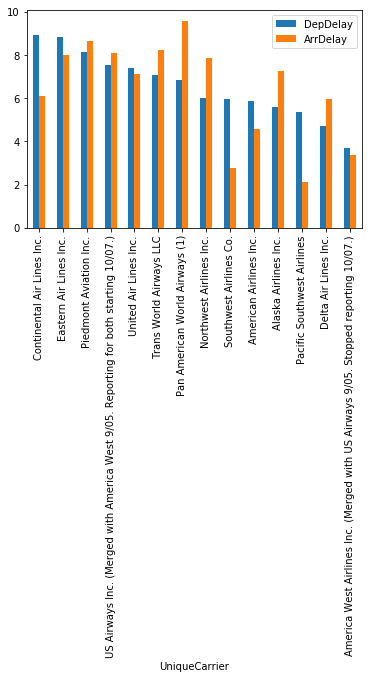
Continental was the worste airline for departures, while PanAm was the worst for arrivals. It looks like some airlines have longer departure delays than arrival delays.

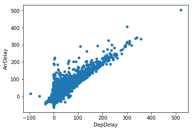
What is the relationship between arrival and departure delays?

df.plot.scatter(x='DepDelay', y='ArrDelay')
plt.show()

outliers = (((df.DepDelay - df.DepDelay.mean()).abs() > df.DepDelay.std()*3) | 
            ((df.ArrDelay - df.ArrDelay.mean()).abs() > df.ArrDelay.std()*3))

sns.lmplot('DepDelay', 'ArrDelay', data=df[~outliers],
           fit_reg=False, hue='UniqueCarrier', scatter_kws={'alpha':0.3})
plt.show()

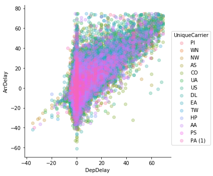
Even after trimming outliers and adding alpha, this chart is too busy.

carrier_averages = df.groupby('UniqueCarrier').agg({'DepDelay':'mean', 'ArrDelay':'mean'}).reset_index()
sns.lmplot('DepDelay', 'ArrDelay', data=carrier_averages,
           fit_reg=False, hue='UniqueCarrier', )
plt.show()

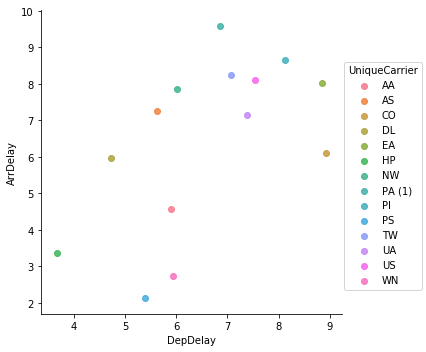
After aggregating by airline it becomes too sparse and loses meaning.

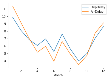
Delays by month

df.groupby('Month').agg({'DepDelay':'mean', 'ArrDelay':'mean'}).plot.line()
plt.show()

df.groupby('Month').agg({'DepDelay':'mean', 'ArrDelay':'mean'}).plot.bar()
plt.show()

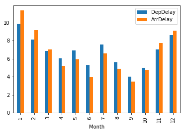
September was the best month to fly, January the worst.

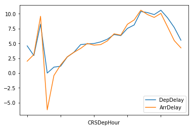
What is the worst time of day to travel?

df['CRSDepHour'] = pd.cut(df.CRSDepTime, list(range(0, 2500, 100)))

df.groupby('CRSDepHour').agg({'DepDelay':'mean', 'ArrDelay':'mean'}).plot()
plt.show()

df.groupby('CRSDepHour').agg({'DepDelay':'mean', 'ArrDelay':'mean'}).plot.bar()
plt.show()

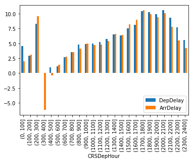
Early morning is the best time to fly, with the delays increasing as the day goes on and peaking around 6pm.

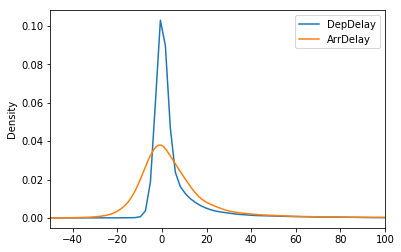
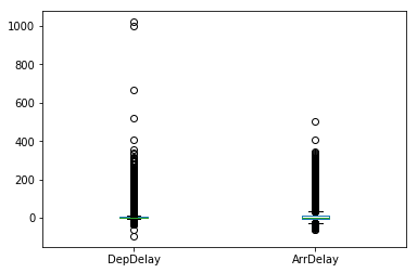
Distribution of Delays

df.loc[:,['DepDelay', 'ArrDelay']].plot.density(xlim=(-50,100))

<matplotlib.axes._subplots.AxesSubplot at 0x1efc8fe6f60>

df.loc[:,['DepDelay', 'ArrDelay']].plot.box()

<matplotlib.axes._subplots.AxesSubplot at 0x1ef963646d8>

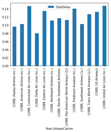
Which Airlines had the most delayed (>15 min) flights

df.groupby(['Year', 'UniqueCarrier']).agg({'DepDelay':lambda x: (x>15).sum()/len(x)}).plot.bar()
plt.show()

Data prepping

Carrier names are going to need some munging.

carriers.loc[carriers.index.intersection(carriers.Description.str.len().nlargest(10).index)]

	Code	Description
9	0GQ	Inter Island Airways, d/b/a Inter Island Air
60	6R	Aerounion Aerotransporte de Carga Union SA de CV
262	B4	Globespan Airways Limited d/b/a Flyglobespan
642	HP	America West Airlines Inc. (Merged with US Air...
690	JAG	JetAlliance Flugbetriebs d/b/a JAF Airservice
720	K3	Venture Travel LLC d/b/a Taquan Air Service
850	MRQ	National Air Cargo Group, Inc.d/b/a Murray Air
1054	QT	Transportes Aereos Mercantiles Panamericanos S.A
1308	US	US Airways Inc. (Merged with America West 9/05...
1460	YAT	Friendship Airways, Inc. d/b/a Yellow Air Taxi

# For simplicity, combine US Air and Amercia West
carriers.loc[[642, 1308], 'Description'] = 'US Airways'

# Drop doing business as (d/b/a) names
drop_dbas = lambda x: str.split(x, 'd/b/a')[0].strip()
carriers['Description'] = carriers['Description'].apply(drop_dbas)

carriers.loc[carriers.index.intersection(carriers.Description.str.len().nlargest(10).index)]

	Code	Description
8	0FQ	Maine Aviation Aircraft Charter, LLC
60	6R	Aerounion Aerotransporte de Carga Union SA de CV
270	BAQ	Aero Rentas De Coahuila S.A. De C.V.
279	BDQ	Aerotaxis De Aguascalientes S.A. De C.V.
294	BIQ	Servicios Aeronauticos Z S.A. De C.V.
302	BNQ	Netjets Large Aircraft Company L.L.C.
323	C5	Commutair Aka Champlain Enterprises, Inc.
1031	PU	Primeras Lineas Uruguays For International
1054	QT	Transportes Aereos Mercantiles Panamericanos S.A
1459	Y8	Yangtze River Express Airlines Company

df['UniqueCarrier'] = df['UniqueCarrier'].map(dict(carriers.values))

df.UniqueCarrier.head()

618384      Piedmont Aviation Inc.
4868305     Southwest Airlines Co.
1455876    Northwest Airlines Inc.
4894209    Northwest Airlines Inc.
4297444       Alaska Airlines Inc.
Name: UniqueCarrier, dtype: object

with open('data/carrier_dict.pkl', 'wb') as file:
    pickle.dump(dict(carriers.values), file)